Autoencoders for anomaly detection

The Phoenix project is focused on the cyber-security of Electrical Power and Energy Systems (EPES). One on the first steps on counter-measuring a cyber-attack is to identify the malicious activity. That task can be addressed by anomaly detection techniques. Artificial Intelligence has proven to be a suitable technology for that task. Deep Learning models, based on convolutional neural networks, can be trained in an unsupervised manner using data from several sensors that monitor the power grid. One family of models to accomplish such a task are the autoencoders: models that are trained to reproduce the input data with little differences respect to the original.
The economic engine of modern society is based in the fast interactions between its members. In this context, there are two key infrastructures that are essential to this society: communications (internet) and transport. The technological developments on both ends allowed the number of daily interactions to grow. Nowadays, the immense amount of such interactions makes management and traceability highly complex tasks. That is one of the reasons why digitalization is on the rise. In the modern society, all these three elements (communication, transport and management) lie upon a common base that enables and supports them: electrical energy.
The power grid is a critical infrastructure for modern society, as it is one of the main gears on its socio-economic engine. Thus, preserving its integrity is a fundamental task. Nowadays the power grid is constantly monitored by multiple sensors that help to detect any potential situations that may occur. The PHOENIX project intends to cast a shield against cyber-attacks on Electrical Power and Energy Systems (EPES) across Europe. One of the tasks on the development of such a tool is to create a system that can detect abnormal activity on the power grid. As it was said on previous entrances of this blog [1], Artificial Intelligence (AI) has proven to be an adequate technology for that assignment. The data from the multiple sensors that are monitoring the EPES can be used to train an AI model based on convolutional neural networks to perform anomaly detection [3].
The convolutional neural networks have proven to be an effective tool at feature extraction. They are widely used for extracting the essential information of data, reducing the dimensionality of the input into a much smaller feature map. Alternatively, the de-convolutional layers can successfully retrace the path and reconstruct the data from a feature map. Such ability enables deep learning models to perform many additional tasks like semantic segmentation and instance segmentation for example. One of the techniques that comes from the “reconstruction” feature of the de-convolutional neural networks is the autoencoder models for anomaly detection. Autoencoding is an unsupervised technique based on extracting a feature map out of a given input data (encode) and then reconstruct it to its original form (decode). During training the network is fed with data from a specific domain and it is asked to learn how to reconstruct the inputs accurately. Once the model is trained, it could recreate a given sample of data with very few differences compared to the original.
Such a model can be used for outlier detection taking advantage of the fact that it is trained on a specific domain. When the model is asked to reconstruct an input data belonging to another domain, it will produce a flawed reconstruction. Effectively measuring the differences between the input and the output allows the model to detect “unexpected” incoming data. For example; let’s imagine that a model was trained with pictures of dogs. If a snake picture is presented to a model fully trained on a dog dataset, it will fail to encode the texture, shape, colour, and any specifics like ears and snout. Thus, the reconstruction will be very different than the original, yielding to a high “difference score” that can be easily spotted by a computer program.
The following figure shows an example of an autoencoder application. The dataset was generated with sine function where Gaussian noise was added on both axes. The figure shows the original input (red) and its reconstruction (blue) for the model trained over different numbers of training rounds (epochs). The progression, from left to right, shows how the autoencoder gets better and better at the reconstruction task.
References
- https://phoenix-h2020.eu/cyber-physical-systems/. Consulted 17th December 2020.
- https://www.freepik.es/fotos-premium/sentado-bernese-mountain-dog-jadeando_8490461.htm. Consulted 17th December 2020.
- Ruoying Wang, Kexin Nie, Tie Wang, Yang Yang, and Bo Long. 2020. Deep Learning for Anomaly Detection. In Proceedings of the 13th International Conference on Web Search and Data Mining (WSDM ’20). Association for Computing Machinery, New York, NY, USA, 894–896. DOI:https://doi.org/10.1145/3336191.3371876
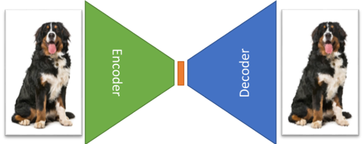
Figure 1: schematics of an autoencoder architecture. Dog picture reference: [1].
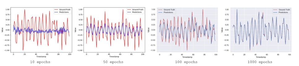
Figure 2: Training examples of an autoencoder. Red line indicates the label (ground-truth value) and the blue one (prediction) is the reconstruction inferred by the model. The figure shows the results of this reconstruction made by models trained during different number of iterations (epochs).
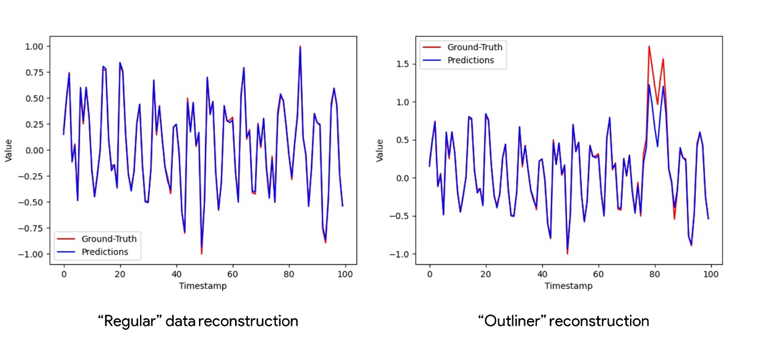
Figure 3: Comparison of an autoencoder model’s performance at reconstruction “normal” data and an outliner. Both left and right show the same signal but the one on the right side was altered to create an anomaly. In that case a pulse was added to the “regular” signal (left). As the “pulsed” signal was unexpected to the model, it was not able to properly reconstruct the signal, generating evident differences between the input and its reconstruction